Reverting to the Mean
As an investor, one would have to value investments across a multiyear holding period. Given that multiples are used for valuation, it is intuitive to expect that lower multiples in a down market would not stay down forever.
To address this, we would have to implement some mechanism to revert to the mean.
Reversion to the mean gives the sense that the difference between the extremes and the average compresses over time, but the sense is incorrect. Values that are far from the average will have to go toward the average, and the values that are close to the average do not show much change.
One Method to Estimate the Rate of Reversion to the Mean
The correlation coefficient (r) is a measure of the linear relationship between two variables. This coefficient will be important to denote the rate of reversion to the mean. The coefficient is calculated from the metric we would like to revert back to the mean.
Correlation Coefficient:
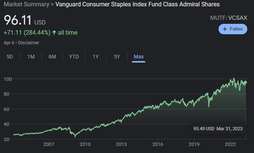
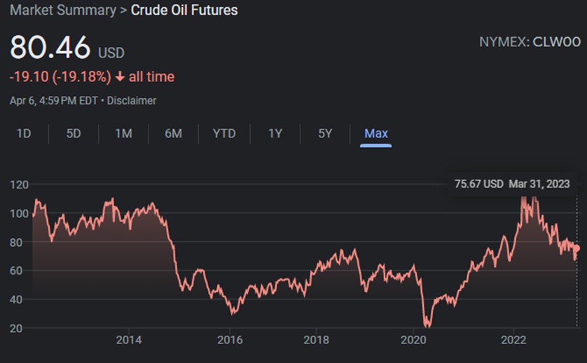
If r is 1.0, there is no reversion to the mean. In other words, the best estimate of the next outcome is simply the past outcome. Higher correlations imply persistence or the existence of skill. In the markets, we would expect a sector with stable demand to have a higher r than a sector exposed to commodity markets.
If r is 0, there is complete reversion to the mean. The best estimate of the next outcome is simply the average.
Let’s look at some index funds to illustrate:
Estimating the Mean:
What is the mean to which the results revert? It depends on how stable the metric is. If the average of the metric has been stable over time, we can use past averages to estimate future averages. If the environment is changing, then we would be cautious to implement such a mechanism. Estimating the mean is difficult because rarely does a valuation metric over time stay stable.
Example Calculation:
With this in mind, we can write down a simple formula to denote an expected outcome:
Expected Metric = r * (Current Metric – Mean) + Mean
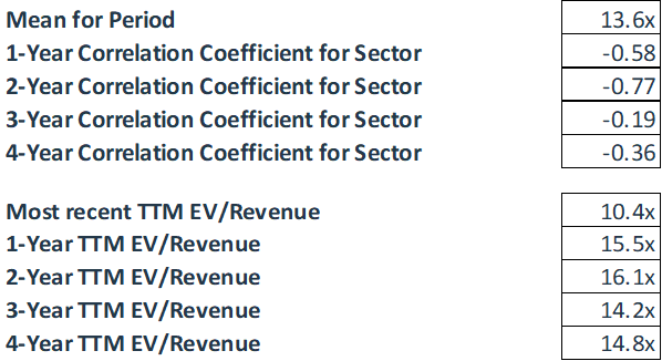
For instance, I have pulled the EV/Revenue multiple for Adobe, Atlassian and Salesforce from 2014 to 2022. The "current" EV/Revenue of Salesforce is 10.4x at the end of December 2022. If we want to estimate the EV/Revenue in four years, we will calculate the four-year correlation coefficient (-0.36) and the mean EV/Revenue (13.6x) for this limited basket of software stocks. Plugging those numbers in we would get:
14.8x = (-0.36) * (10.4x – 13.6x) + 13.6x
Note that this is not a prediction about Salesforce. It delineates what happens, on average, to (ideally) a large sample of companies in the same sector that possess similar EV/Revenue multiple profiles.
This analysis and simple exercise is inspired by the current market’s skittish environment. Note that this formula is quite rough and I will be exploring how to improve it.